Welcome readers to another adventure in metropolitan building permit plotting. If that doesn’t get you going, you might be at the wrong link…Two weeks ago we explored Seattle. Today it’s Denver. Both cities are high-growth options for coastal refugees. Denver offers another study in how single family markets evolve in the face of substantial economic and population growth.
Above and beyond the economic lessons, the benefits of this study relevant to R users are as follows:
- Wrangling a mess of single excel files pulled from the internet into a tidy format
- This post will provide hints for those curious about geocoding on a budget. As many in the
Rcommunity know, certain API limits can make geocoding a bit more difficult. If you’d like specifics, reach out on Twitter. - The regex here is strong, if I may say. Cleaning addresses and extracting our geographic information required extensive regexing. It isn’t always the most efficient, but it got the job done.
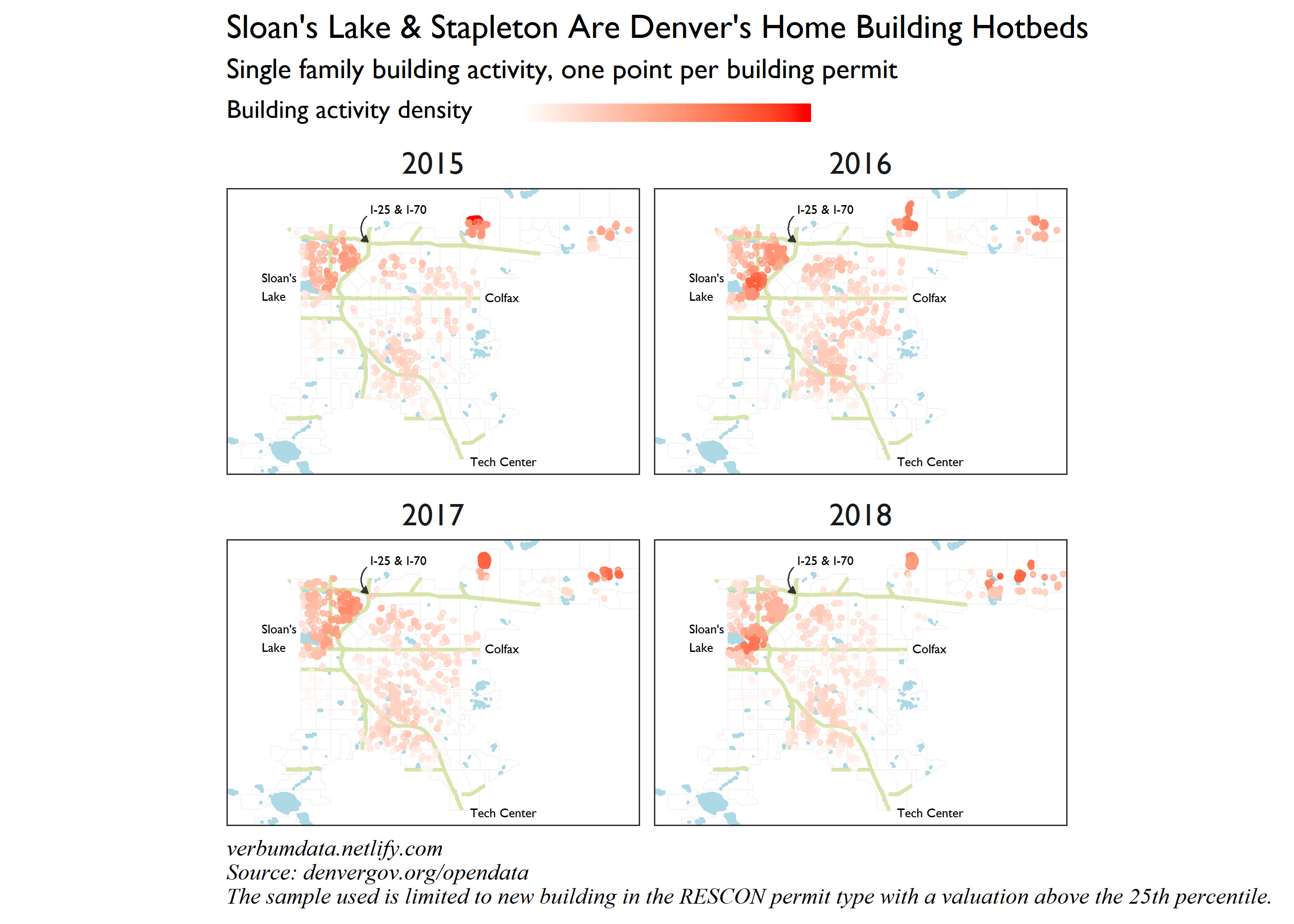
Here is our final plot to pique your interest. The data we study here is building permit applications in Denver for (mostly) residential properties. The idea is to understand how and where single family building activity has occurred in the recent past.
Accessing and assessing the data
We must begin, as usual, with option setting and library imports.
library(tidyverse); library(rvest)
library(readxl); library(janitor)
library(lubridate); library(tigris)
library(sf)

extrafont::loadfonts(device = "win")
options(tigris_use_cache = TRUE, tigris_class = "sf")
Unlike our Seattle experience, Denver does not provide easy API access to their building permit data. In fact, the open data portal is nearly useless! I can recommend to those interested in finding Denver data this site instead.
With the source established, I was dismayed to discover that the building permit data was locked in dozens of excel files. To access everything I first had to locate it. The following chunk undertakes that work. This method allows us to access the excel files without having to download and store them on disk, which is nice.
# the major links first
root_link <- "https://www.denvergov.org/"
website <- read_html("https://www.denvergov.org/content/denvergov/en/denver-development-services/help-me-find-/building-permits.html")

# burrow in and find the good (bad?) stuff

permit_links <- website %>%
  html_nodes("li") %>%
  html_nodes("a") %>%
  html_attr("href") %>%
  .[grepl("\\.xls|\\.xlsx", .)] %>%
  gsub(root_link, "", .)

# now a for loop to collect everything

raw_excel <- list()

for(i in seq_along(permit_links)){
  temp <- tempfile()
  download.file(paste0(root_link, permit_links[i]),
                mode = "wb",
                destfile = temp)
  raw_excel[[i]] <- read_excel(temp) %>%
    clean_names()

  unlink(temp)
  print(i)
}
Good gracious. But the dirty work is not over. One delight in collecting dirty metro area data is finding bizarre inputs. A bit of exploratory data analysis showed that ONE file (!!!) among the whole collection was accidentally uploaded in a different format. Actually, I would have preferred all files come in the Dec. 2016 format, but alas.
In any case, a function to clean the raw excel input was necessary.
# write function to clean excel sheets

clean_denver_permit <- function(excel){
  if(ncol(excel) == 22) { # almost all sheets have 22 columns
    mydf <- excel %>%
      row_to_names(2) %>% # grab the second row and clean the names
      clean_names() %>%
      select(-starts_with("na")) %>% # a bit dangerous, but this kicks out "na" cols
      filter(!is.na(date_issued),
             !is.na(permit_number)) %>%
      mutate(date_issued = as.Date(as.numeric(date_issued), origin = "1899-12-30"),
             valuation = as.numeric(valuation),
             permit_fee = as.numeric(permit_fee)) %>%
      rename(original_address = address, subtype = location) %>%
      filter(!is.na(original_address))

  } else { # this is for the one accidental export with fewer cols
    mydf <- excel %>%
      clean_names() %>%
      select(-c(stat_code, final_date, date_received, bid_auth_name,
                log_number, exempt, co_required, date_co_issued, cancel)) %>%
      select(-starts_with("na")) %>%
      mutate(date_issued = as.Date(date_issued),
             valuation = as.numeric(valuation),
             permit_fee = as.numeric(permit_fee)) %>%
      rename(original_address = address, subtype = location) %>%
      filter(!is.na(original_address))
  }
  return(mydf)
}

# denver permits list to data frame

dpldf <- map_df(raw_excel, clean_denver_permit)dpldf## # A tibble: 271,333 x 10
## date_issued permit_number original_address subtype class units valuation
## <date> <chr> <chr> <chr> <chr> <chr> <dbl>
## 1 2019-01-28 2019-MECH-00~ 180 N Cook ST 5~ //505 Repa~ <NA> 4260
## 2 2019-01-28 2018-RESCON-~ 10275 E 59th Av~ //SFR New ~ <NA> 276752.
## 3 2019-01-28 2018-RESCON-~ 1633 S Clayton ~ // New ~ 1 432889
## 4 2019-01-28 2019-RESCON-~ 10288 E 57th Ave // New ~ 1 205730
## 5 2019-01-28 2019-RESCON-~ 10000 E 59th Dr // New ~ 1 218852
## 6 2019-01-28 2019-RESCON-~ 9964 E 60th Ave // New ~ 1 221267
## 7 2019-01-28 2019-RESCON-~ 9954 E 60TH // New ~ 1 242894
## 8 2019-01-28 2019-RESCON-~ 9952 E 60th Ave // New ~ 1 250342
## 9 2019-01-28 2019-RESCON-~ 9972 E 60th Ave // New ~ 1 254891
## 10 2019-01-28 2019-RESCON-~ 10308 E 57th Ave // New ~ 1 274626
## # ... with 271,323 more rows, and 3 more variables: permit_fee <dbl>,
## # owners_name <chr>, contractors_name <chr>Now that is something we might be able to use, once we’ve processed it, of course.
Data processing gets its own header
The purpose of the next cleaning was to extract relatively clean addresses for geocoding.
Any analyst faced with loosely structured building permit data has my sincerest pity. The addresses in this data set were formatted variously. Some addresses had “detached garage” written into them, others included work process numbers. You’ll note, there was NO ZIP CODE information. Geocoding looked difficult.
Only a full-frontal regex assault could save the day. So full frontal that I had to run the scrub twice. If any reader can think of a faster way to accomplish this task, please let me know.
The thorny issue was that some of the regex’s change the structure of the data. In other words, removing a word on the first pass might reveal a trailing digit, which, on the second pass, will be removed. I tried custom ordering the regex patterns but to no avail.
The to_remove vector collects a majority of the undesirable or irrelevant words.
# we will need to remove these words

to_remove <- paste("garage", "basement", "unit", "addition",
                   "sfr", "mod", "n/a", "fence", "[0-9] unit",
                   "bldg", " ?pav.*$", "bsmt", "\\s+det\\s+",
                   "detached\\s+[sg]", "elec", "bath", "\\d+$",
                   "gar$", "clubhouse", "[^[:graph:][:space:]]",
                   "residence", "pergola", "shoring", "\\#",
                   "rm", "none", "\\*failed to decode utf16\\*",
                   "rear deck", "deck", "\\d+\\s+&.?\\s*\\d+[a-z]?",
                   "podium to", "\\w+\\s*&\\s*\\w","&$",
                   sep = "|")
With the regex removal established, it was time to apply it to the data. Once we accomplish the cleaning we could extract the individual addresses for residences to input into our geocoder.
# drop any items without addresses, remove extra numbers, clean up labels,
# delete trailing digits in address

dp_proc <- dpldf %>%
  mutate_if(is.character, tolower) %>%
  mutate(class = trimws(gsub("[[:digit:]]...", "", class)),
         class = trimws(gsub(" ?/ ?", "/", class)),
         class = case_when(
           class == "change of use only" ~ "change of use",
           class == "addition to building" ~ "addition",
           TRUE ~ class),
         permit_type = gsub("[^[:alpha:]]", "", permit_number),
         original_address = trimws(str_remove_all(original_address, to_remove)),
         original_address = str_remove_all(original_address, to_remove), # repeat
         original_address = gsub("  ", " ", original_address),
         address = paste0(trimws(original_address), " denver, co"),
         single = str_extract(original_address, "^\\d+\\s*[a-z]\\s*\\w+"))

# create vector of unique residential, new building addresses

resi_address <- dp_proc %>%
  filter(class %in% "new building",
         permit_type %in% "rescon") %>%
  distinct(address, .keep_all = TRUE) %>%
  group_by(single) %>%
  summarize(actual = str_extract(address, "^\\d+\\s*[a-z]\\s*\\w+\\s\\w+\\s")[1]) %>%
  mutate(actual = ifelse(is.na(actual),
                         paste0(single, " denver, co"),
                         paste0(actual, "denver, co")))
Geocoding on a budget with a regex adventure
Many are aware that Google changed API access terms last year. The wonderful ggmap package was hobbled by a daily API limit (up to 2000 before billing begins). The intrepid (or broke) in need of a world class geocoder can still use Google, though. The cunning will guess the process, but for those curious, reach out on Twitter and we can chat.
Most important, Google + clever regex allowed us to map a majority of the residential permits to their geographic location. I won’t pretend this process is fail proof, but given the quality of the input data, I’m delighted to have made it this far.
# note that the object web_text does not exist here...
# for those curious, reach out and we can chat

locations_regex <- str_extract_all(web_text, "...(?<=\\[{3})(\\d+.*?\\d+,-\\d+.\\d+.*?denver, co)") %>%
  unlist() %>%
  .[!grepl('NA denver',.)]
With the mysterious geocoding done, now behold the creation of a lookup table we can use to map the addresses and coordinates to the original addresses from our processed data frame.
address_lookup <- tibble(
  address =
    str_extract_all(locations_regex, '(?<=[\\"])\\d+\\b\\s+\\w+(.)*co') %>%
    unlist(),
  lat_long =
    str_extract_all(locations_regex, '(?<=\\[{3})(\\d+.*?\\d+,-\\d+.\\d+)') %>%
    unlist()
  ) %>%
  separate(lat_long, into = c("lat", "lon"), sep = ",", convert = TRUE)
The lookup table is complete. We can now join onto the original data frame and clean up further before our cartographic activity begins.
rp <- dp_proc %>%
  left_join(address_lookup, by = "address") %>%
  filter(class %in% "new building",
         permit_type %in% "rescon",
         !valuation %in% c(0, NA)) %>%
  distinct(date_issued, original_address, valuation, .keep_all = TRUE) %>%
  mutate(subtype = gsub("\\W+$|^\\W+\\d+", "undefined", trimws(subtype)),
         subtype = gsub("[^[:alpha:][:space:]]", "", trimws(subtype)),
         subtype = case_when(
             grepl("garage|gar", subtype,) ~ "garage",
             grepl("undefined", subtype) ~ "undefined",
             grepl("unit", subtype) ~ "unit",
             grepl("duplex", subtype) ~ "duplex",
             grepl("sfr|house|residence", subtype) ~ "residence",
             grepl("sud", subtype) ~ "sewer",
             TRUE ~ subtype),
         subtype = ifelse(subtype == "", "undefined", trimws(subtype)),
         year = year(date_issued))
Cartographic violence?
APIs would have made our path to this point cleaner. Nevertheless we arrived at a (relatively) clean data set and set our sights on collecting the geographic information needed to plot Denver’s permit data. Readers be advised: here I import only rds files created from the shp file sources. Those in need of the shp files should follow the lead of the great James Bain. You can find the links to the necessary files here. To parse the Census files for the highways, refer to this document.
# retrieve tract-level census shape files

denver_map <- tigris::tracts(state = "CO",
                             county = "denver",
                              cb = TRUE)

# read in other features
# hwy filtered only for road type I and U

den_hwy <- readRDS("../../static/2019-02-09_den-hwy.rds")

den_lakes <- readRDS("../../static/2019-02-09_den-lakes.rds")

# set boundaries

map_box <-  c(xmin = -105.13, ymin = 39.6, xmax = -104.7, ymax = 39.82)
hwy_sub <- st_crop(den_hwy, map_box)
county_sub <- st_crop(denver_map, map_box)
lakes_sub <- st_crop(den_lakes, map_box)
We will again make use of Kamil Slowikowski’s density function to understand where building permit activity is most concentrated in Denver.
# helpful density function
get_density <- function(x, y, ...) {
  dens <- MASS::kde2d(x, y, ...)
  ix <- findInterval(x, dens$x)
  iy <- findInterval(y, dens$y)
  ii <- cbind(ix, iy)
  return(dens$z[ii])}

# create the final data frame needed for mapping

rpsf <- rp %>%
  drop_na(lat, lon) %>%
  filter(year < 2019) %>%
  st_as_sf(coords = c("lon", "lat"),
                 crs = 4326) %>%
  group_by(year) %>%
  mutate(lon_dense = map_dbl(seq_along(geometry), ~ geometry[[.x]][1]),
         lat_dense = map_dbl(seq_along(geometry), ~ geometry[[.x]][2]),
         density = get_density(lon_dense, lat_dense)) %>%
  filter(lat_dense < 39.81,
         subtype %in% c("residence", "duplex", "undefined"),
         valuation > quantile(valuation, 0.25))
Long suffering readers! Rest assured. You have toiled to this point and will be rewarded with an actual plot. The nastiness ensues below. I’d highlight the legend tinkering as the item which I expect to use most in the future. Playing with location, margins, justification, and more was no easy task.
# plot

ggplot() +
  geom_sf(data = county_sub, color = "grey95",
          fill = NA, alpha = 0.5, size = 0.2) +
  geom_sf(data = lakes_sub, fill = "lightblue",
          color = "lightblue") +
  geom_sf(data = hwy_sub, color = "#d7e5ac",
          size = 0.7) +
  geom_point(data = rpsf,
            aes(x = lon_dense, y = lat_dense,
                color = density, alpha = 1),
            size = 0.8) +
  annotate("text",
           x = -104.988, y = 39.805,
           label = "I-25 & I-70",
           color = "black",
           family = "Gill Sans MT",
           size = 1.8, hjust = 0) +
  annotate("text",
           x = -105.09, y = 39.7487582,
           label = "Sloan's\nLake",
           color = "black",
           family = "Gill Sans MT",
           size = 1.8, hjust = 0) +
  annotate("text",
           x = -104.88, y = 39.741,
           label = "Colfax",
           color = "black",
           family = "Gill Sans MT",
           size = 1.8, hjust = 0) +
  annotate("text",
           x = -104.894045, y = 39.6224321,
           label = "Tech Center",
           color = "black",
           family = "Gill Sans MT",
           size = 1.8, hjust = 0) +
  geom_curve(data = county_sub,
             aes(x = -104.991, y = 39.80, xend = -104.99, yend = 39.781),
             color = "#353535", size = 0.3, ncp = 10,
             arrow = arrow(type = "closed",
                           length = unit(0.1, "cm"))) +
  scale_color_gradient2(low = "white", high = "red") +
  scale_x_continuous(expand = c(0,0)) +
  scale_y_continuous(expand = c(0,0)) +
  facet_wrap(~ year) +
  coord_sf(datum = NA) +
  guides(size = FALSE, alpha = FALSE,
         color = guide_colorbar(
           direction = "horizontal",
           ticks = FALSE, barheight = 0.5,
           barwidth = 8, label = FALSE,
           title.position = "left",
           title.vjust = 1.31, title.hjust = 0)) +
  theme_bw() +
  theme(text = element_text(family = "Gill Sans MT"),
        plot.caption = element_text(hjust = 0, face = "italic"),
        strip.text = element_text(size = 12),
        strip.background = element_blank(),
        axis.title = element_blank(),
        legend.text = element_blank(),
        legend.title = element_text(size = 10),
        legend.position = "top",
        legend.justification = "left",
        legend.margin = margin(2, 0, -10, 0)) +
  labs(title = "Sloan's Lake & Stapleton Are Denver's Home Building Hotbeds",
       subtitle = "Single family building activity, one point per building permit",
       color = "Building activity density    ",
       caption = "Source: denvergov.org/opendata\nThe sample used is limited to new building in the RESCON permit type with a valuation above the 25th percentile.")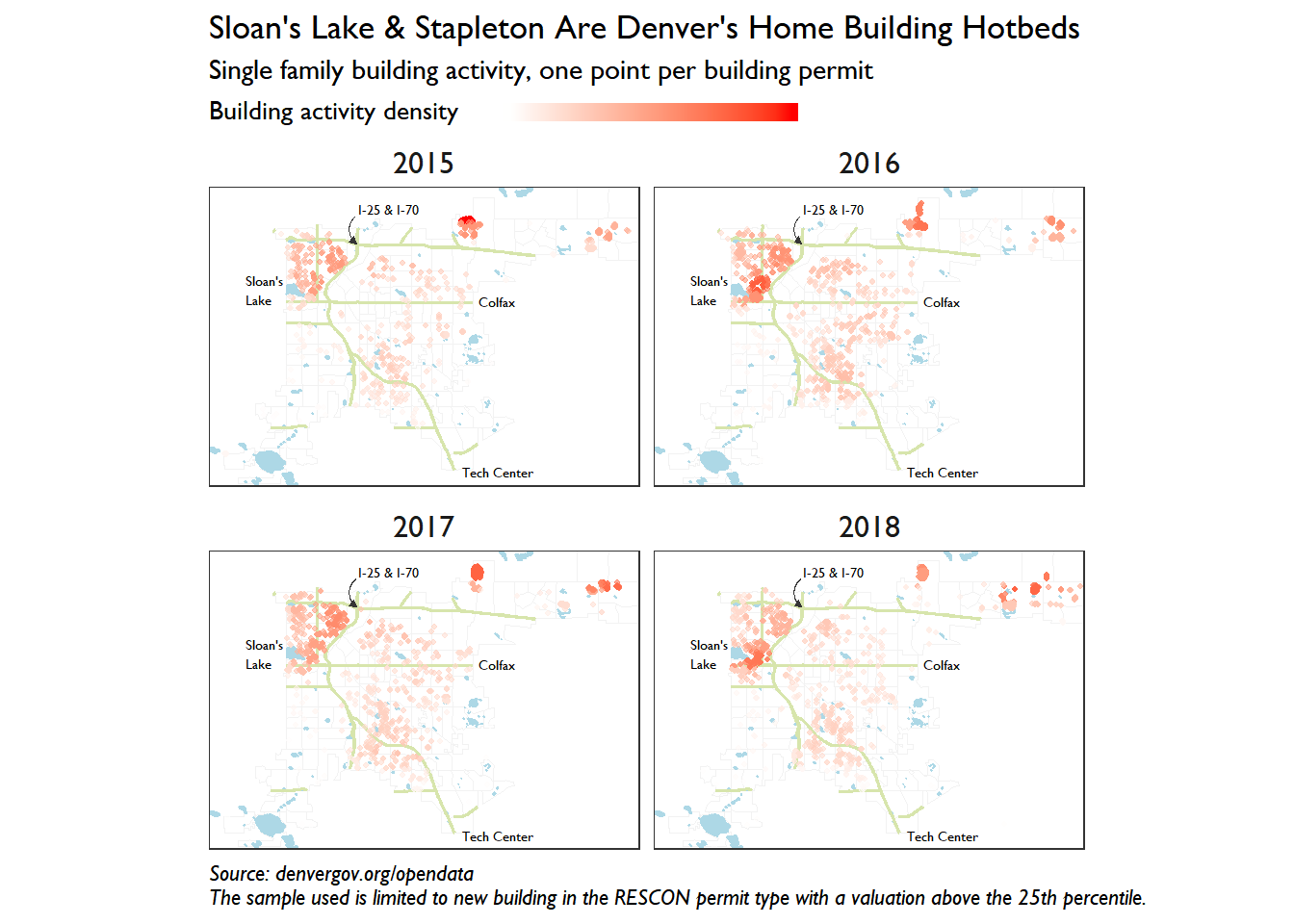
What can we say about Denver’s building activity as a result of our hard work? The obvious insights made it into the plot title. Sloan’s Lake and Stapleton are alive and well in the single family building world. The next item to note is the evolution around Sloan’s Lake over the past 4 years. Activity has moved south and west since 2015 and found a new verve in 2018. Who said Denver stopped growing?
Finally, Denver city dwellers would be wise to keep their eyes trained east. Impressive build outs are underway in Northfield, Montbello, and Green Valley ranch. Stop by on your way to DIA and scrutinize the true face of urban expansion.